library(dplyr)

bfi[c("agree", "consc", "extra", "neuro", "open")] %>%
  cov(use = "pairwise") %>%
  diag() %>%
  sqrt()
agree consc extra neuro open
0.8984019 0.9513469 1.0609041 1.1963314 0.8083739 %>%R’s native pipe operator, |>, was only introduced in R 4.1. Before that, we used the analogous operator provided by the dplyr package, %>%. The dplyr pipe is almost exactly the same as the base R version. For example, we can re-create our first motivating example as follows.
library(dplyr)
bfi[c("agree", "consc", "extra", "neuro", "open")] %>%
cov(use = "pairwise") %>%
diag() %>%
sqrt() agree consc extra neuro open
0.8984019 0.9513469 1.0609041 1.1963314 0.8083739 For most practical purposes, the Base R and dplyr pipes are interchangeable, but there are a few minor differences between |> and %>%. For example, the dplyr pipe uses the . character as the dataset placeholder symbol.
mtcars %>%
  lm(mpg ~ hp + disp, data = .) %>%
  summary()
Call:
lm(formula = mpg ~ hp + disp, data = .)

Residuals:
    Min      1Q  Median      3Q     Max
-4.7945 -2.3036 -0.8246  1.8582  6.9363

Coefficients:
             Estimate Std. Error t value Pr(>|t|)
(Intercept) 30.735904   1.331566  23.083  < 2e-16 ***
hp          -0.024840   0.013385  -1.856 0.073679 .
disp        -0.030346   0.007405  -4.098 0.000306 ***
---
Signif. codes:  0 '***' 0.001 '**' 0.01 '*' 0.05 '.' 0.1 ' ' 1

Residual standard error: 3.127 on 29 degrees of freedom
Multiple R-squared:  0.7482,    Adjusted R-squared:  0.7309
F-statistic: 43.09 on 2 and 29 DF,  p-value: 2.062e-09
The dplyr pipe also allows more flexible usage of the dataset placeholder symbol.
mtcars %>%
  lm(mpg ~ hp + disp, data = ., weights = .$wt) %>%
  summary()
Call:
lm(formula = mpg ~ hp + disp, data = ., weights = .$wt)

Weighted Residuals:
   Min     1Q Median     3Q    Max
-7.873 -3.313 -1.434  3.071 10.635

Coefficients:
             Estimate Std. Error t value Pr(>|t|)
(Intercept) 29.510142   1.329831  22.191  < 2e-16 ***
hp          -0.022962   0.011752  -1.954 0.060426 .
disp        -0.027690   0.006297  -4.398 0.000135 ***
---
Signif. codes:  0 '***' 0.001 '**' 0.01 '*' 0.05 '.' 0.1 ' ' 1

Residual standard error: 5.114 on 29 degrees of freedom
Multiple R-squared:  0.7511,    Adjusted R-squared:  0.7339
F-statistic: 43.75 on 2 and 29 DF,  p-value: 1.749e-09
mtcars |>
lm(mpg ~ hp + disp, data = _, weights = _$wt) |>
summary()Error in summary(lm(mpg ~ hp + disp, data = mtcars, weights = "_"$wt)): invalid use of pipe placeholder (<input>:3:0)%$%The exposition pipe, %$%, is a very useful flavor or pipe operator provided by the magrittr package. The exposition pipe offers an elegant alternative to the dataset placeholder symbol in many common types of pipeline. Most notably, pipelines involving functions that employ the so-called formula interface, such as lm(), t.test(), or boxplot().
Instead of passing the processed dataset into the first argument of a downstream function, the exposition pipe exposes the column names of the processed data frame to the downstream function. For example, the following code uses the exposition pipe to regress age on extra in the bfi data.
library(magrittr)

bfi %$% lm(extra ~ age + open)
Call:
lm(formula = extra ~ age + open)

Coefficients:
(Intercept)          age         open
   2.752007     0.004406     0.276073
The exposition pipe allows the lm() call to access the column names of bfi when resolving the model formula extra ~ age. We can achieve analogous results in several ways.
# Explicitly regress vectors:
lm(bfi$extra ~ bfi$age + bfi$open)
Call:
lm(formula = bfi$extra ~ bfi$age + bfi$open)

Coefficients:
(Intercept)      bfi$age     bfi$open
   2.752007     0.004406     0.276073
# Use the Base R equivalent of %$%:
with(bfi, lm(extra ~ age + open))
Call:
lm(formula = extra ~ age + open)

Coefficients:
(Intercept)          age         open
   2.752007     0.004406     0.276073
# Use a dataset placeholder symbol:
bfi |> lm(extra ~ age + open, data = _)
Call:
lm(formula = extra ~ age + open, data = bfi)

Coefficients:
(Intercept)          age         open
2.752007 0.004406 0.276073 Use the bfi dataset and an exposition pipe to create a pipeline to draw a conditional boxplot that visualizes the distribution of agree scores within gender groups.
boxplot() function to draw the plot.library(magrittr)
bfi %$% boxplot(agree ~ gender)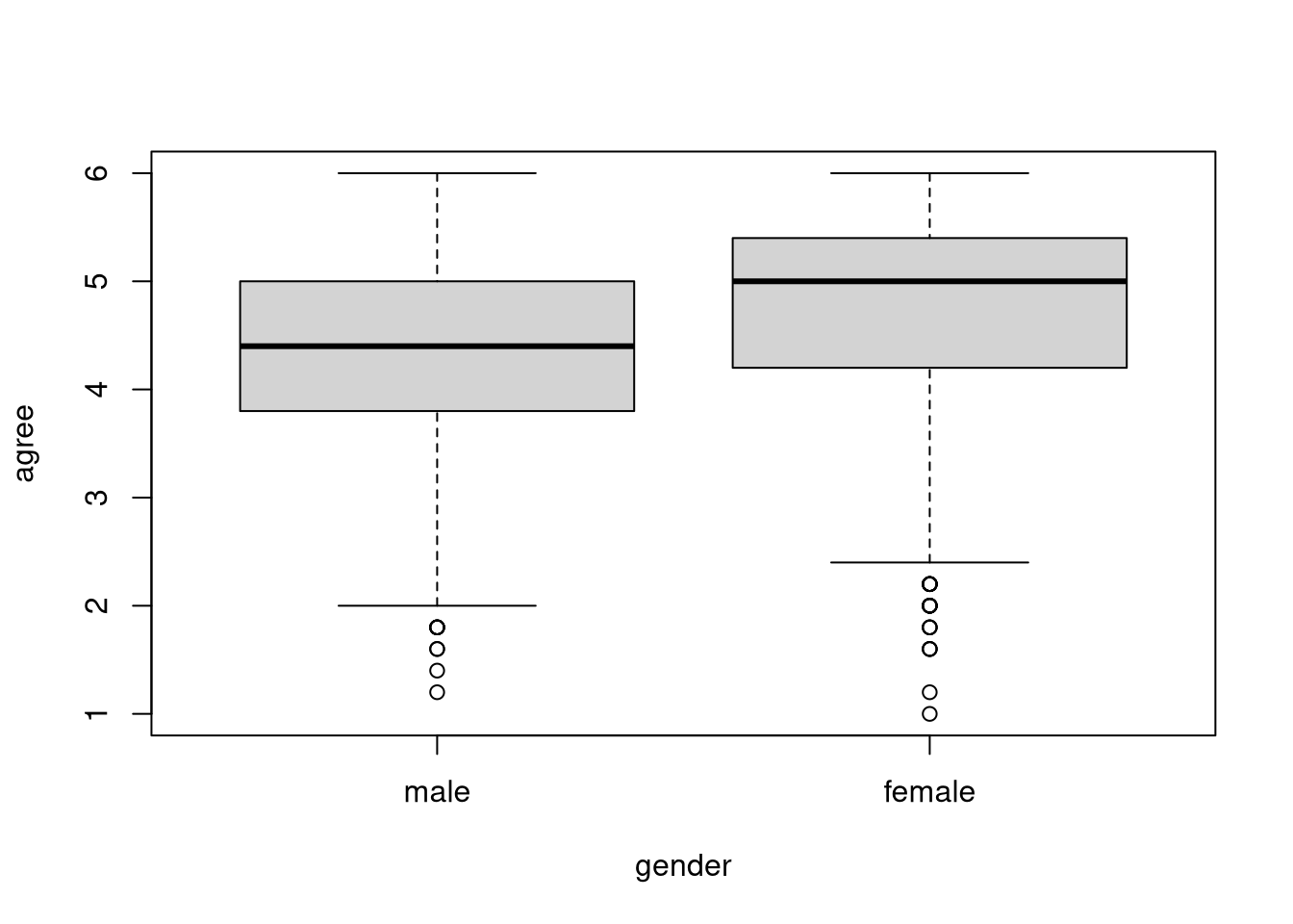
Create a pipeline that includes at least on exposition pipe to perform the following operations with the bfi dataset:
dplyr::slice_sample().agree onto extra, open, and gender.
lm().library(dplyr)
set.seed(235711)
bfi |>
slice_sample(n = 500) %$%
lm(agree ~ extra + open + gender) |>
resid() |>
abs() |>
sum()[1] 318.6229%<>%The final type of pipe that we’ll cover is certainly a niche tool, but it provides a nice little bit of syntactic sugar. We only care about assignment pipes in particular types of pipelines. Names, pipelines with two characteristics:
For example, the following pipeline uses dplyr data manipulation functions to modify the bfi1 dataset and overwrite the original with the modified version produced by the pipeline.
bfi1 <- bfi
head(bfi1)
a1 a2 a3 a4 a5 c1 c2 c3 c4 c5 e1 e2 e3 e4 e5 n1 n2 n3 n4 n5 o1 o2 o3 o4
61617 2 4 3 4 4 2 3 3 4 4 3 3 3 4 4 3 4 2 2 3 3 6 3 4
61618 2 4 5 2 5 5 4 4 3 4 1 1 6 4 3 3 3 3 5 5 4 2 4 3
61620 5 4 5 4 4 4 5 4 2 5 2 4 4 4 5 4 5 4 2 3 4 2 5 5
61621 4 4 6 5 5 4 4 3 5 5 5 3 4 4 4 2 5 2 4 1 3 3 4 3
61622 2 3 3 4 5 4 4 5 3 2 2 2 5 4 5 2 3 4 4 3 3 3 4 3
61623 6 6 5 6 5 6 6 6 1 3 2 1 6 5 6 3 5 2 2 3 4 3 5 6
o5 gender education age agree consc extra neuro open
61617 3 male <NA> 16 4.0 2.8 3.8 2.8 3.0
61618 3 female <NA> 18 4.2 4.0 5.0 3.8 4.0
61620 2 female <NA> 17 3.8 4.0 4.2 3.6 4.8
61621 5 female <NA> 17 4.6 3.0 3.6 2.8 3.2
61622 3 male <NA> 17 4.0 4.4 4.8 3.2 3.6
61623 1 female some_college 21 4.6 5.6 5.6 3.0 5.0bfi1 <- bfi1 %>%
slice_sample(n = 20) %>%
select(-matches("\\d$"))
head(bfi1) gender education age agree consc extra neuro open
1 male graduate_degree 38 5.2 5.8 5.2 1.0 4.8
2 male some_college 27 4.2 5.4 3.8 3.0 3.4
3 female college_graduate 20 5.2 3.8 4.6 3.8 5.2
4 male some_college 40 5.6 5.0 4.6 1.4 4.6
5 male some_college 26 5.0 5.2 3.8 2.2 4.2
6 female college_graduate 27 5.6 5.0 4.8 1.6 5.0The assignment pipe cleans up the syntax a little but and makes the destructive nature of the pipeline clear. When you see an assignment pipe, you know that the modified data produced by the pipeline will replace the original dataset.
bfi1 <- bfi
head(bfi1)
a1 a2 a3 a4 a5 c1 c2 c3 c4 c5 e1 e2 e3 e4 e5 n1 n2 n3 n4 n5 o1 o2 o3 o4
61617 2 4 3 4 4 2 3 3 4 4 3 3 3 4 4 3 4 2 2 3 3 6 3 4
61618 2 4 5 2 5 5 4 4 3 4 1 1 6 4 3 3 3 3 5 5 4 2 4 3
61620 5 4 5 4 4 4 5 4 2 5 2 4 4 4 5 4 5 4 2 3 4 2 5 5
61621 4 4 6 5 5 4 4 3 5 5 5 3 4 4 4 2 5 2 4 1 3 3 4 3
61622 2 3 3 4 5 4 4 5 3 2 2 2 5 4 5 2 3 4 4 3 3 3 4 3
61623 6 6 5 6 5 6 6 6 1 3 2 1 6 5 6 3 5 2 2 3 4 3 5 6
o5 gender education age agree consc extra neuro open
61617 3 male <NA> 16 4.0 2.8 3.8 2.8 3.0
61618 3 female <NA> 18 4.2 4.0 5.0 3.8 4.0
61620 2 female <NA> 17 3.8 4.0 4.2 3.6 4.8
61621 5 female <NA> 17 4.6 3.0 3.6 2.8 3.2
61622 3 male <NA> 17 4.0 4.4 4.8 3.2 3.6
61623 1 female some_college 21 4.6 5.6 5.6 3.0 5.0bfi1 %<>%
slice_sample(n = 20) %>%
select(-matches("\\d$"))
head(bfi1) gender education age agree consc extra neuro open
1 female some_college 27 5.6 5.6 5.8 2.2 5.8
2 female some_college 51 5.4 5.6 4.2 4.4 4.2
3 male high_school_graduate 49 4.0 3.4 4.0 3.0 4.4
4 female high_school_graduate 19 3.8 3.8 2.0 3.6 3.8
5 female some_college 27 4.6 5.8 6.0 4.2 5.8
6 female some_college 26 5.0 5.8 4.4 1.0 5.0Note that we must use the dplyr pipe, %>%, if we include an assignment pipe in our pipeline. The Base R pipe doesn’t play nicely with the assignment pipe. More specifically, the assignment pipe behaves like a basic pipe (i.e., |> or %>%) when combined with the Base R pipe operator, as you can see below.
bfi1 <- bfi
head(bfi1)
a1 a2 a3 a4 a5 c1 c2 c3 c4 c5 e1 e2 e3 e4 e5 n1 n2 n3 n4 n5 o1 o2 o3 o4
61617 2 4 3 4 4 2 3 3 4 4 3 3 3 4 4 3 4 2 2 3 3 6 3 4
61618 2 4 5 2 5 5 4 4 3 4 1 1 6 4 3 3 3 3 5 5 4 2 4 3
61620 5 4 5 4 4 4 5 4 2 5 2 4 4 4 5 4 5 4 2 3 4 2 5 5
61621 4 4 6 5 5 4 4 3 5 5 5 3 4 4 4 2 5 2 4 1 3 3 4 3
61622 2 3 3 4 5 4 4 5 3 2 2 2 5 4 5 2 3 4 4 3 3 3 4 3
61623 6 6 5 6 5 6 6 6 1 3 2 1 6 5 6 3 5 2 2 3 4 3 5 6
o5 gender education age agree consc extra neuro open
61617 3 male <NA> 16 4.0 2.8 3.8 2.8 3.0
61618 3 female <NA> 18 4.2 4.0 5.0 3.8 4.0
61620 2 female <NA> 17 3.8 4.0 4.2 3.6 4.8
61621 5 female <NA> 17 4.6 3.0 3.6 2.8 3.2
61622 3 male <NA> 17 4.0 4.4 4.8 3.2 3.6
61623 1 female some_college 21 4.6 5.6 5.6 3.0 5.0bfi1 %<>%
slice_sample(n = 20) |>
select(-matches("\\d$")) gender education age agree consc extra neuro open
1 male college_graduate 30 4.0 3.4 4.2 3.6 4.4
2 female high_school_graduate 41 5.4 5.0 5.2 3.6 3.6
3 female <NA> 16 4.6 4.6 2.6 3.6 4.0
4 male some_college 18 3.0 3.2 4.8 1.6 5.4
5 female graduate_degree 25 5.4 2.0 5.6 4.4 5.2
6 female some_college 21 5.0 4.8 4.6 2.6 3.4
7 female college_graduate 41 5.2 5.8 3.4 5.2 3.6
8 female some_college 23 4.0 5.4 1.8 6.0 5.8
9 female college_graduate 27 1.6 3.0 1.2 2.4 5.4
10 female some_college 21 5.4 2.2 3.8 1.2 3.4
11 female some_college 44 5.4 4.8 5.4 4.2 4.4
12 female some_college 52 4.2 4.0 5.0 1.0 4.8
13 female some_college 23 5.2 5.0 5.8 1.8 5.0
14 female some_college 27 5.0 4.6 3.4 3.6 3.6
15 male some_college 60 4.8 4.6 4.4 2.4 4.0
16 female high_school_graduate 25 5.0 4.4 5.2 5.0 4.2
17 male college_graduate 26 4.4 4.0 5.4 1.4 4.4
18 male some_high_school 35 5.0 4.6 4.0 3.2 5.4
19 male some_college 24 4.0 3.2 4.6 2.0 4.2
20 female high_school_graduate 46 4.0 5.4 4.2 2.8 3.2head(bfi1) a1 a2 a3 a4 a5 c1 c2 c3 c4 c5 e1 e2 e3 e4 e5 n1 n2 n3 n4 n5 o1 o2 o3 o4 o5
1 3 4 4 2 6 5 3 5 5 5 2 5 4 5 5 3 3 5 5 2 6 2 4 5 5
2 2 5 5 6 6 6 4 5 3 1 1 3 5 6 5 4 5 5 3 1 4 5 5 5 5
3 1 5 5 3 4 4 5 5 2 3 5 5 4 1 4 3 3 4 4 4 5 4 2 5 2
4 3 4 2 2 3 3 2 2 4 1 2 2 5 4 5 2 3 1 1 1 6 3 6 5 1
5 2 6 5 5 6 3 1 3 5 6 1 1 6 6 4 4 4 6 4 4 5 4 6 6 1
6 1 6 4 5 4 5 5 5 1 4 3 3 5 5 5 3 4 2 2 2 4 6 4 5 4
gender education age agree consc extra neuro open
1 male college_graduate 30 4.0 3.4 4.2 3.6 4.4
2 female high_school_graduate 41 5.4 5.0 5.2 3.6 3.6
3 female <NA> 16 4.6 4.6 2.6 3.6 4.0
4 male some_college 18 3.0 3.2 4.8 1.6 5.4
5 female graduate_degree 25 5.4 2.0 5.6 4.4 5.2
6 female some_college 21 5.0 4.8 4.6 2.6 3.4Use the assignment pipe to create a pipeline that implements the following operations:
mtcars dataset.mtcars dataset with the standardized version.You can use the scale() function to standardize variables.
library(magrittr)

mtcars %<>% scale()
We can sanity check the results by computing the means and variances of each variable.
colMeans(mtcars) mpg cyl disp hp drat
7.112366e-17 -1.474515e-17 -9.085614e-17 1.040834e-17 -2.918672e-16
wt qsec vs am gear
4.682398e-17 5.299580e-16 6.938894e-18 4.510281e-17 -3.469447e-18
carb
3.165870e-17 apply(mtcars, 2, var) mpg cyl disp hp drat wt qsec vs am gear carb
1 1 1 1 1 1 1 1 1 1 1 Looks good!