In a Quarto document, code chunks are self-contained blocks of executable code embedded within the text. They serve as the fundamental bridge between the narrative and computational parts, and they enable a seamless integration of analysis and exposition. Each chunk is delimited by a specific syntax (for example, triple backticks followed by a language label such as {r}) that tells Quarto which language engine to use. When the document is rendered, Quarto evaluates these chunks in the specified language environment, captures their outputs—such as console text, tables, plots, or other visualizations—and inserts them directly into the document at the chunk’s position. This workflow supports the principles of literate programming and reproducible research, ensuring that results are dynamically linked to the underlying code rather than being static artifacts.
Conceptually, Quarto treats code chunks as part of a larger computational document graph. During rendering, Quarto manages execution order, variable environments, and inter-chunk dependencies to maintain consistency. This means that chunks are not merely snippets of text to be formatted; they are active components in the document’s computational state. For instance, a variable created in one chunk can be referenced and used in another, allowing for modular, incremental development of analyses. Quarto also provides mechanisms for caching, error handling, and execution control, giving users flexibility in how computation is performed during document compilation.
Importantly, code chunks are not limited to R. They can be written in Python, Julia, or other supported languages within the same document. This multilingual capability makes Quarto a versatile platform for mixed-language workflows, which are increasingly common in data science and applied research.
Example
First chunk:
# Create a small datasetset.seed(123)data <-data.frame(group =rep(c("A", "B"), each =10),score =c(rnorm(10, mean =75, sd =5),rnorm(10, mean =82, sd =6)))# Display a quick summary of the datasummary(data$score)
   Min. 1st Qu.  Median    Mean 3rd Qu.    Max.
  68.67   73.58   78.91   79.31   84.22   92.72
In the first chunk, we see a dataset being generated and stored. Next, we see that the summary of this dataset is being requested. When rendering the document, the output of this request is automatically being printed in the document (as you can see printed directly below the code chunk).
Second chunk:
# Use the dataset created in the previous chunkmodel <-lm(score ~ group, data = data)# Display regression resultssummary(model)
Call:
lm(formula = score ~ group, data = data)

Residuals:
     Min       1Q   Median       3Q      Max
-13.0514  -3.3335   0.1264   2.1877   9.4697

Coefficients:
            Estimate Std. Error t value Pr(>|t|)
(Intercept)   75.373      1.754  42.970  < 2e-16 ***
groupB         7.879      2.481   3.176  0.00523 **
---
Signif. codes:  0 '***' 0.001 '**' 0.01 '*' 0.05 '.' 0.1 ' ' 1

Residual standard error: 5.547 on 18 degrees of freedom
Multiple R-squared:  0.3591,    Adjusted R-squared:  0.3235
F-statistic: 10.09 on 1 and 18 DF,  p-value: 0.005231
The second chunk takes the dataset that was stored in the first chunk and performs some additional analysis on this, which is again printed directly below the chunk. This illustrates the dependencies between separate code chunks.
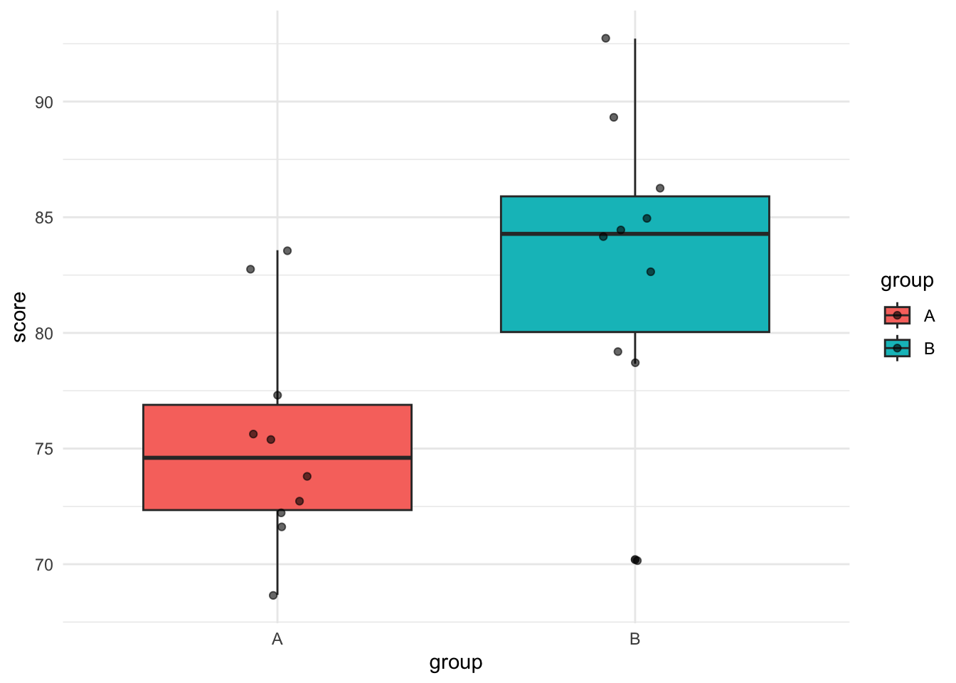
Third chunk:
Distribution of scores by group.
The third chunk again illustrates this dependency, and in addition also shows that code can be executed that creates visualizations, which are then also directly executed and printed in the document.
Together, these three chunks illustrate that:
Each chunk is executed in the same R session, meaning objects like data and model persist across chunks.
Output is automatically captured and displayed, first as numerical summaries, then as model output, and finally as a plot.